By: Rosina Savisaar
In the February 2022 issue of the RNA Journal, we describe our recent work applying the NETseq (Native Elongating Transcript sequencing) method to Drosophila embryos (dNETseq). dNETseq is a technique for sequencing nascent RNAs, that is to say, incomplete RNAs that are still in the process of being synthesized. How can we specifically capture nascent RNA, given that it only makes up a small proportion of the RNA in the cell? The trick used in the dNETseq approach is to capture the RNA polymerase by targeting it with antibodies. Unlike mature RNAs, nascent RNAs are physically attached to the polymerase, and will therefore be isolated along with it. We then sequence roughly the final 100 nucleotides of these nascent RNA molecules, corresponding to the last segment of RNA transcribed by the RNA polymerase (Pol II).
By seeing where the 3’ ends of the reads map, we can locate Pol IIs across the genome with single-nucleotide precision. To facilitate this type of analysis, the reads are processed to only leave the position of the last nucleotide. When such data is visualized in a genome browser, it has a strikingly discrete appearance: long stretches with barely any reads are interrupted by short regions containing dense clusters of reads piled on top of each-other. An example can be seen in Figure 1 for a portion of the Grunge (Gug) gene, visualized using the Integrative Genomics Viewer (IGV).
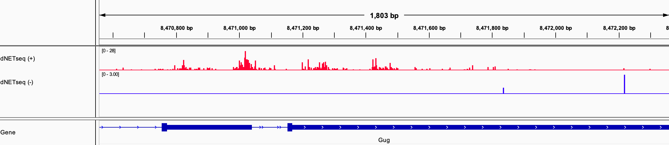
Figure 1: dNETseq data from 4-6 hour old Drosophila melanogaster embryos. Antibodies specific to the Ser5P phosphoisoform of Pol II were used.
How should we interpret this landscape? Most intuitively, these pile-ups of reads correspond to regions where Pol II is slowed down or even paused – the longer it takes Pol II to slog its way through a given sequence region, the more likely we are to capture it at that location, leading to a higher read density. However, other interpretations are also possible. Most notably, because the antibodies used in the dNETseq experiment are specific to particular phosphoisoforms of the Pol II C-terminal domain (CTD), the clusters could also correspond to phosphorylation hotspots.
What-ever the biological interpretation of these peaks and valleys, this topology should be accounted for in our analysis. In other words, we want to convert the numerical counts of reads at different positions to a binary classification, where the transcriptome would be divided into valleys (large regions with few reads) and peaks (short regions with many reads). The difficulty lies in deciding how many reads should count as “few” or “many”. Even if reads were positioned completely randomly, one would sometimes expect to find several of them clustered around the same position, simply through chance. Therefore, the threshold read density for labelling a region as a peak should require a number of reads that is sufficiently high that it is unlikely to occur just through chance co-occurrence of reads.
In bioinformatics, the process of automatically identifying peak regions is referred to as “peak calling”. Peak calling methods have been most extensively developed for the analysis of Chromatin Immunoprecipitation sequencing (ChIP-seq) data (e.g. MACS2). Similarly to dNETseq, ChIP-seq data also has a ‘lumpy’ appearance. For ChIP-seq data, these lumps are usually interpreted as positions where a protein of interest binds to DNA. Put simply, most ChIP-seq peak callers select a threshold and then apply it to the genome, labelling regions with read densities above the threshold as peaks, potentially adjusting the threshold to account for sequencing or mapping biases within different genome regions.
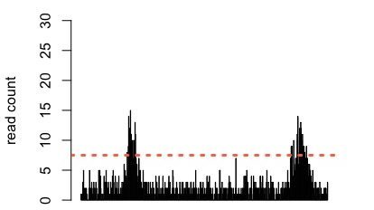
Figure 2: Simulated data showing two regions with an accumulation of reads. A threshold is applied (orange dashed line) and regions where the read density exceeds the threshold are called as peaks.
However, the superficial similarities between ChIP-seq and dNETseq data belie a crucial difference. ChIP-seq is based on DNA sequencing, whereas in dNETseq, it is RNA that is sequenced. The amount of RNA molecules present in the cell varies between genes, as not all genes are expressed at the same level. Therefore, what counts as a high or a low read density will differ based on the expression level of the gene, as the more a gene is expressed, the more readily we obtain reads from it. The threshold for calling a peak should thus be set independently for each transcript, in accordance with its level of expression.
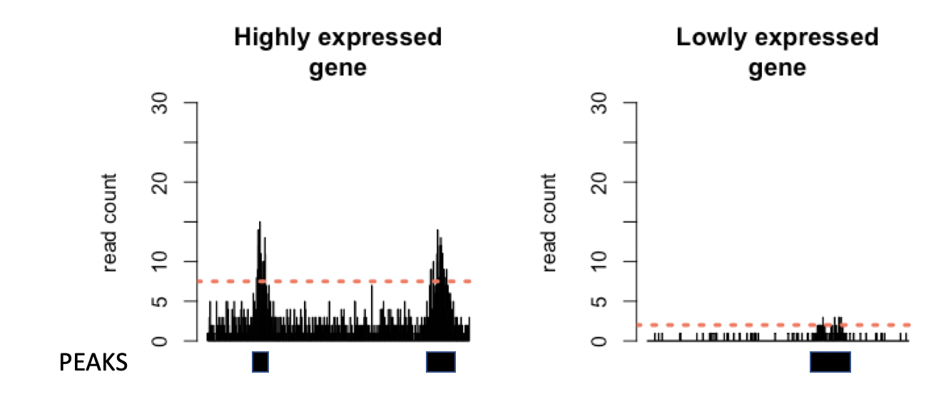
Figure 3: Simulated data for a highly and a lowly expressed gene. The threshold for calling a region as a peak (orange dashed line) is higher in the more highly expressed gene, to account for higher background read density.
This problem is not unique to dNETseq. Rather, it appears when-ever peak calling is applied to RNA-seq data, such as in Crosslinking and Immunoprecipitation sequencing (CLIP-seq). In CLIP-seq data, the peaks are interpreted as corresponding to the binding sites of a particular RNA-binding protein. Although this is biologically quite a different problem from that solved using dNETseq, the formal similarity is such that it should be possible to call peaks in dNETseq data using a simple peak caller designed for CLIP-seq data. In this project, we decided against this strategy and instead chose to develop our own peak caller specifically for dNETseq data so as to have full flexibility in designing its behavior.
The key problem to solve for any peak caller is that of how to determine the threshold for calling a peak as significant. In our peak caller, the number of dNET-seq reads mapping to a transcript is used as a proxy for its transcription initiation rate. Specifically, for each transcript, we perform a simulation where we randomize the positions of the reads mapping to the transcript, maintaining the total number of reads. From this simulation, we can see the read densities expected by chance alone, given the total read count of the transcript. We set the threshold at the 99th percentile of the obtained distribution of read counts per position, calling regions as peaks if the read count in the real data surpasses this threshold.
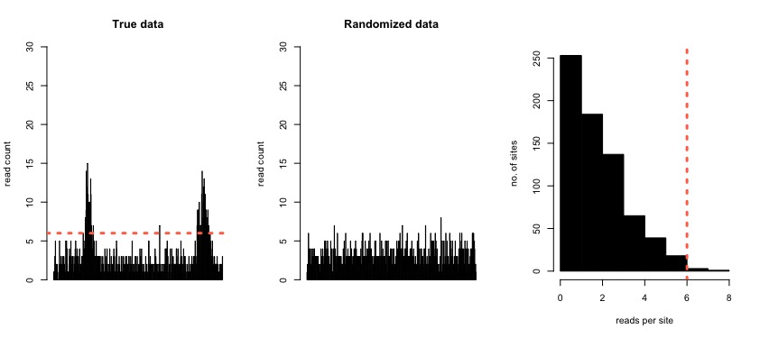
Figure 4: Simulated data with two regions that are enriched for reads (left). In the middle panel, the same region is shown with the reads redistributed randomly. The panel on the right shows the distribution of the number of reads per site in the randomized data. The 99th percentile of this distribution is used as the peak calling threshold with the real data (orange dashed line in the left-most and right-most panels).
So far, our strategy is identical to certain CLIP-seq peak callers, most notably that of Yeo et al. 2009. However, we have built upon this simple approach in several ways. Firstly, as Pol II pausing is expected to occur over a region of several adjacent nucleotides, we were interested in capturing not single significant positions but rather whole regions with an increased read density. Hence, instead of labelling each position with its own read count, we have labelled it with the mean read density of a sliding window of nucleotides centred on that position. The size of this window can be specified by the user. Note that at the very edges of the transcription unit, edge effects may arise and so it is best to be careful in the interpretation of peaks very close to the transcription start or end site. For our own analyses, this problem did not arise because we always exclude the first and the terminal exons of the gene from analysis in any case, as their mechanisms of splicing may differ from those of internal exons.
Secondly, we were worried that our strategy may lead to artificial interdependencies between peaks. Namely, when determining whether or not a given region counts as a peak, the threshold used will depend on the read density in the rest of the transcript. If the transcript contains other large peaks, then this will push up the total read density and thus slightly increase the threshold. As a result, the more regions of increased read density occur in the transcript, the less likely it is that any one of them would be called as a peak. This was concerning for us, as we were interested in the relationships between peaks within the same exon. For instance, if an exon has a peak at the very start, does that mean that it is less likely to have peaks in the middle? Such questions were important to us, as the peaks potentially represent splicing-related pausing. We thus implemented a setting whereby the threshold for calling a peak was set separately for each intron-exon pair (the exon and the intron immediately upstream, if present), by using only the rest of the transcript and not the intron-exon pair itself when determining the empirical threshold. This way, no artificial interdependencies are introduced within the relevant region.
Thirdly, certain positions can appear with a high coverage of reads not for any biological reason but because of biases in PCR amplification. Such positions qualitatively differ from presumed biological peaks, as they appear as a single site with an accumulation of reads, rather than several neighboring positions with increased read density. Hence, we discard peaks where 90% or more of the contributing reads derive from the same position (this threshold can be adjusted). Some of the other user-adjustable parameters include the minimum number of reads per peak, the minimum length of a peak, and the required proximity between two peaks for them to be merged into one.
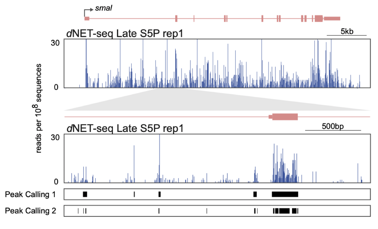
Figure 5: An extract from our publication (Figure 4A prepared by Pedro Prudêncio), showing peaks called in dNETseq data with different settings. The track Peak Calling 1 uses a sliding window size of 21 nucleotides, requires a minimum of 10 reads per peak and merges peaks if they are within 21 nucleotides of each-other. The track Peak Calling 2 uses a sliding window size of 5 nucleotides, requires a minimum of 5 reads per peak and merges peaks if they are within 5 nucleotides of each-other.
The most important test of any such algorithm is whether garbage input produces garbage output – in other terms, that the method itself is not leading to the emergence of artifactual patterns. In order to generate such garbage input, we randomized the positions of the reads within each transcript, and then ran our peak caller using such randomized reads. We then plotted out average peak densities across the first 100 nucleotides of exons. We found that whereas real reads led to highly structured patterns, the garbage input led to what effectively looked like garbage.
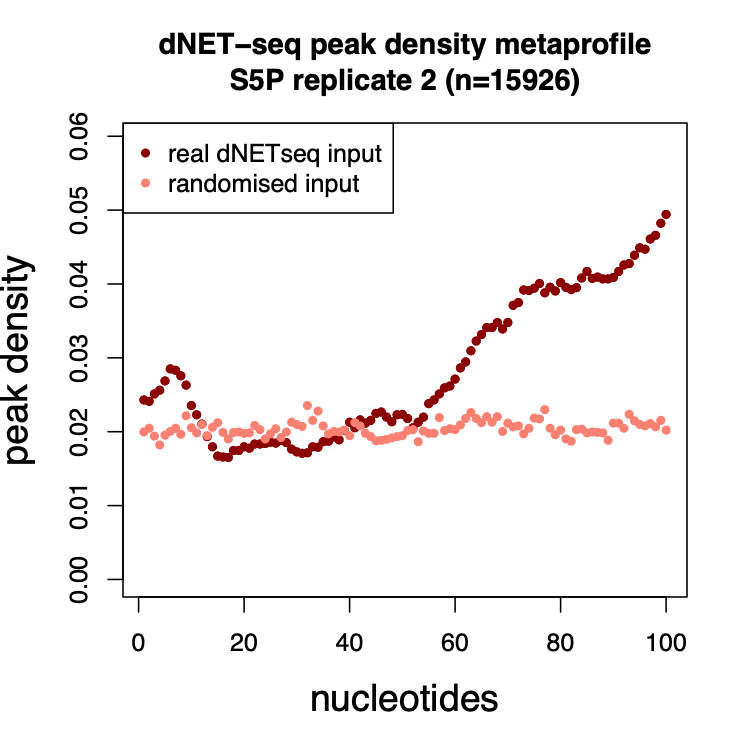
Figure 6: Mean peak density per position (relative to the 3’ splice site) for real dNETseq data and for the randomized control.
We made the decision not to publish the peak caller as a polished software package with all the bells and whistles, simply because that would have meant less time for going after biological questions. However, the source code is freely available to anybody. Drop us a line if you would like our help to get it up and running for yourselves!
This project has received funding from the European Union’s Horizon 2020 research and innovation programme under grant agreement no. 842695 (Marie Skłodowska-Curie Actions).